In this article, I am going to show you how to make instant multiplication table in Microsoft Excel. As I said in the previous guides, Excel worksheets are the best place to make our mathematical calculations and official accounting. Now here I am showing you one of the essential calculation which uses for students of primary classes. Now in Microsoft Excel, it will be made easily by more than two ways, but I will show you just two of them. The first method of making this table is directly typing and selecting them for copyright. And the second way is using a smooth formula then applying for all of them.
Make Instant Multiplication Table in Microsoft Excel 2016
Make Instant Multiplication Table
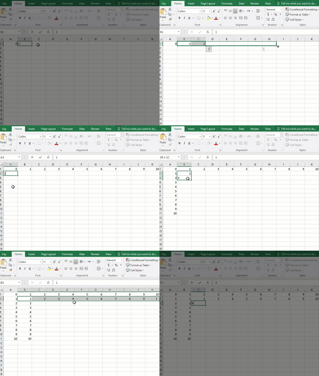
Step 1. Through this step, you are going to learn how to easy type and make instant multiplication table in Excel worksheets. You can make or use this method on your notebook also Or in your classroom for your students by using the calculator or your brain. Through this method at first, open your Excel application and in cells write from Zero to Ten from right left side to right. Then also from that zero to ten from top to below. Then put the cursor then write one, and on the below and right side of number one write two. Watch this GIF to understand quickly how to type them easily.
Now when you wrote like this, here where I wrote FOUR, Here to continue typing and making the table. You should not type the same number here you need to multiply 2×2 and write the result which is four. And continue like this the others also. And also continue according to the GIF to make it smooth like this
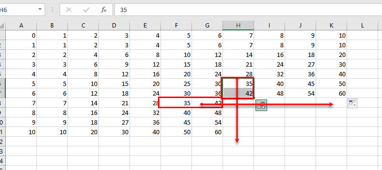
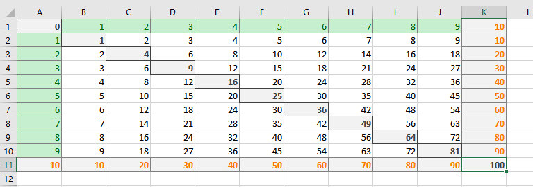
Continue like this at the end you can get your table. It was the first way for making an instant multiplication table. But because it takes more time and to make it quickly use the next step by using formula.
Make Instant Multiplication Table Using Formula
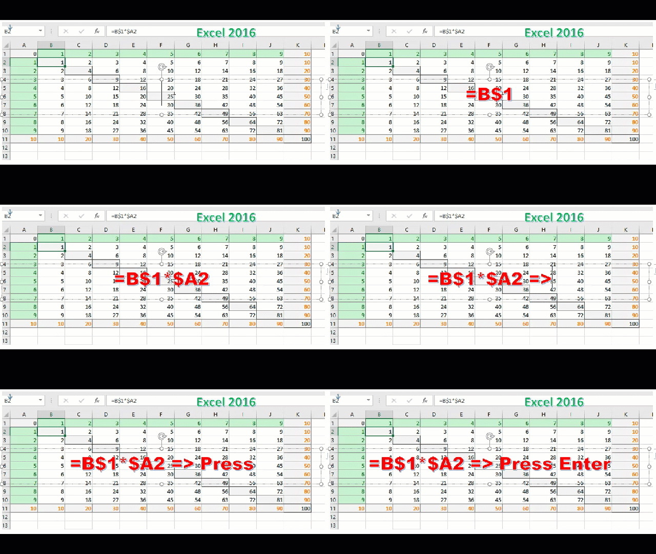
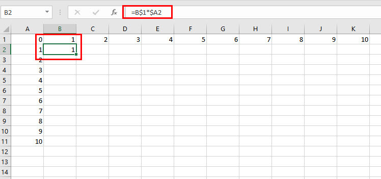
Step 2. Through this step, you can use one smooth formula for making this table. To make this table by using formula open your Excel workbook, and write again from Zero to Ten from left to right side and from top to the below. Then put your cursor on the cell B2. Here you need to write this formula =B$2*$A2 then Click enter. To type this formula at first, click type the equation sign ( = ), then click on the cell B2 where is written number one (1). To change it to B$2 press on the button FN and F4 at the same time. When you pressed the first time it will change to $B$2, Press these two keys again to change it to B$2. Now type the multiplication sign (*) and click on A2. Here also you need to change it to $A2, again do the same process on them by clicking tree times on FN+F4 then click enter.
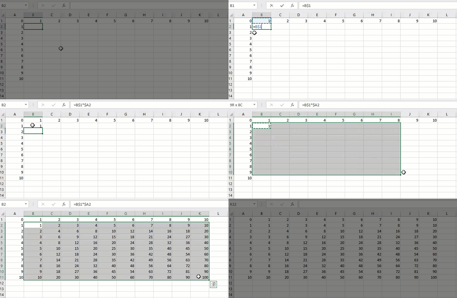
Now you have typed the formula, and here in the picture, you see the result and also the method. Now through to this GIF, you learn how to do the process quickly and make our table. Here it’s simple, copy the first result and select all cells from right side till to ten and from top to below till the ten then click ENTER.
Here you have don and made your table now use it and make your table design it.
Conclusion
It’s all about how to make instant multiplication table in Microsoft Excel 2016. Building this table is simple as other tables into future tables again we have some more difficult tables and system of accounting which will be useable in shops, markets, libraries, and else more centres and companies.
And it was the first time to show how to do correctly. The task or type the formula in Excel, by GIF. Because in Microsoft Excel and again Microsoft Excess we need some time for good understanding to use from GIF. Thanks for being with us.
Related contents:

Leave a Reply